UNIT B| Analytical Tools

In a free market , all price movement comes down to a supply and demand equation. As mentioned in Unit A, the same principle is valid for currencies: more demand indicates scarcity and leads to higher prices, while weaker demand means lower prices. At the same time, more supply and abundance leads to lower prices and less supply makes prices increase.

In this context, it is usually said that fundamentals are what drives prices up and down defining supply and demand. Fundamentals are excellent for developing an overall picture of the markets, sure, but still it's just a complementary perspective, and by no means the only one.

Conventional wisdom tells us that a wide gulf separates the theories forwarded by academic economists and the day-to-day of those who trade the markets. When approaching fundamental analysis from a practical perspective, as we shall do in this chapter, the wide gulf emerges as an unbridgeable gap.

If the principle mentioned at the start is true, then why do we periodically witness an increase in demand while prices escalate higher? According to the theory, it should be the other way round. In this chapter we examine whether or not traders can work around this apparent contradiction.

Many researchers agree that the disjunction actually exists: exchange rates exhibit volatility and persistent misalignments which seem largely unconnected to macroeconomic fundamentals. In this sense, we will examine how this comes to be and display a series of guidelines to make fundamental analysis operational for traders.

As a starting point, a basic understanding of the different models used in fundamental analysis will be conveyed. Then, we will guide you through explanations on how to use this type of analysis to get a long-term view of where prices are heading, as well as some hints on how to use it for near term forecasting. And finally, a totally different perspective on fundamentals will be disclosed.

We deliver the know-how and you only have to decide if the resources provided are useful or not for you. Do we have a deal? Great, let's proceed!

1. Basic Theories Of Fundamental Analysis

One of the dominant debates among financial analysts is the relative validity of the two primary approaches of analyzing markets: fundamental and technical analysis. There are several points of distinction between fundamentals and technicals but it's true that both study the causes of market movements and both attempt to predict price action and market trends. Fundamentals, our main subject in this chapter, focus on financial and economic theories, as well as political developments to determine forces of supply and demand.

In general, the exchange rate of a currency versus other currencies is a reflection of the condition of that country's economy, compared to the other countries' economies. This assumption is based on the belief that the exchange is determined by the underlying health of the two nations involved in the pair.

When evaluating one nation's currency relative to another, fundamental analysis relies upon a broad understanding of multi-national macroeconomic statistics and events. Usually it examines core underlying elements that influence the economy of a particular currency. These might include, on the one hand, economic indicators such as interest rates, inflation, unemployment, money supply and growth rates. On the other hand, it also examines socio-political conditions which could impact on the level of confidence in a nation's government and affect the climate of stability.

Several experts agree on the fact that fundamental analysis is more effective in predicting trends for the long-term (one year or more), while technical analysis is more appropriate for shorter time scales and intraday trading. Nonetheless, empirical evidence from the previous chapter reveals that technical analysis is also capable of identifying long-term trends. Moreover, in this chapter we will prove that fundamental factors do trigger short-term developments on which you can capitalize.
Our aim is to leave you with an understanding of both types of analysis even if you prefer one or the other as your primary tool to make your trading decisions.

Fundamental analysts use different models to examine currency values and forecast future movements. Herewith we describe the major models for forecasting currency prices, their principles and limitations.

Purchasing Power Parity

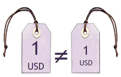
The purchasing power parity model is based on the theory that exchange rates between currencies are in equilibrium when their purchasing power is the same in each of the two countries. An increase in a country's domestic price level means a change in its inflation rate. When this happens, the inflation rate is expected to be offset by an equivalent but opposite change in the exchange rate. According to the purchasing power parity model, if the value of a hamburger, for instance, is 2USD in the US and 1GBP in the UK, then the GBP/USD exchange rate must be 2USD per 1GBP (GBP/USD 2.0000).
What if the actual interbank exchange rate displays GBP/USD 1.5000? In this case the Pound Sterling would be considered undervalued and the US Dollar overvalued.

Therefore, according to this model the two currencies should move towards the 2:1 ratio which is the price difference that same goods in both countries have. This also means that when a country's inflation is rising, the exchange rate for its currency should depreciate in relation to other currencies, in order to return to parity.

In the absence of transportation and other transaction costs such as tariffs or taxes, competitive markets should theoretically equalize the price of an identical good in two countries (with prices expressed in the same currency). But in reality such costs exist and influence the cost of goods and services, and therefore should be considered when weighing prices. Unfortunately the purchasing power parity model does not reflect those costs when determining the exchange rates, being this its major weakness. Another weakness is the fact that the model only applies for goods and ignores services. Furthermore, other factors such as inflation and interest rate differentials impacting exchange rates, are not taken into account in this model.

Interest Rate Parity

The interest rate parity model is based on the concept that when a currency experiments appreciation or depreciation against another currency, this imbalance must be brought to equilibrium by a change in the interest rate differential.

The parity is needed to avoid an arbitrage condition with a risk-free return. Theoretically, it works like this: you borrow money in one currency, then exchange that currency for another currency in order to invest in interest-bearing instruments. At the same time you purchase futures contracts to convert the currency back at the end of the holding period. The amount should be equal to the returns from purchasing and holding similar interest-bearing instruments of the first currency. An arbitrage would occur if the returns for both transactions were different, thus producing a risk-free return.

Let's see with an example: supposing the USD has a 5% annual interest rate and the AUD 8%, the exchange rate is AUD/USD 0.7000, and the forward exchange rate implied by a contract maturing in 12 months is AUD/USD 0.7000. It is obvious that Australia has a higher interest rate than the US. The arbitrage consists in borrowing in the country with a lower interest rate and invest in the country with a higher interest rate. All else being equal, this would help you make money without any risk. A Dollar invested in the US at the end of the 12-month period will be:

1 USD X (1 + 5%) = 1.05 USD

and a Dollar invested in Australia (after conversion into AUD and back into USD at the end of the 12-month period will be:

1 USD X (0.7/0.7)(1 + 8%) = 1.08 USD

The arbitrage would work as follows:

1. Borrow 1 USD from the US bank at 5% interest rate.

2. Convert USD into AUD at current spot rate of 0.7000 AUD/USD giving 1.4285 AUD.

3. Invest the 1.4285 AUD in Australia for the 12 month period.

4. Purchase a forward contract on the 0.7000 AUD/USD (that is, covering your position against exchange rate fluctuations).

And at the end of the 12-month period:

1. 1.4285 AUD becomes 1.4285 AUD (1 + 8%) = 1.5427 AUD

2. Convert the 1.5427 AUD back to USD at 0.7000 AUD/USD, giving 1.0798 USD

3. Pay off the initially borrowed amount of 1 USD to the US bank with 5% interest, that is, 1.05 USD

The resulting arbitrage profit is 1.0798 USD − 1.0500 USD = 0.0298 USD, which is almost 3 cents of profit per each USD.

The basic idea behind the arbitrage pricing theory is the law of one price, which states that 2 identical items will be sold for the same price and for if they do not, then a riskless profit could be made by arbitrage: buying the item in the cheaper market then selling it in the more expensive market.
But contrary to the theory, arbitrage opportunities of this magnitude vanish very quickly because a combination of some of the following events occurs and reestablishes the parity: the US interest rates can go up, the forward exchange rates can go down, the spot exchange rates can go up or the Australian interest rates can go down.
As we have seen in recent years during the Carry Trade, currencies with higher interest rates have characteristically appreciated rather than depreciated on the reward of future containment of inflation and of a higher yielding currency. This is the reason why this model alone is not useful either.

International Balance of Payments Model

Until the 90's the balance of payments theory focused primarily on the balance of trade, a sub account of the current account. This was due to the fact that capital flows were not as significant as nowadays and the trade balance made up the major part of the balance of payments for most world economies.

Under this model, a nation with a trade deficit will experience a reduction of its foreign exchange reserves it used to pay for the imported goods, as we have seen when we explained the trade balance in the video of Chapter A02. A country has to change its own currency for the exporters currency to pay for the goods - this makes its own currency depreciate.
In turn a cheaper currency makes the nation's exported goods and services less expensive in the global market place while making imports more expensive. The simplified balance of payments model states that after an intermediate period, imports are forced down and exports rise, thus stabilizing the trade balance and the currency towards equilibrium.

Based on this model, many analysts forecast that the USD would fall in value against other major currencies, specially the Euro, due to the expanding US trade deficit. But in reality, international capital flows in the last decade have been characterized by global investors acquiring billions of assets in the US, yielding a net capital account surplus. This surplus, despite of statistical discrepancies and currency fluctuations, balanced the current account deficit.

Since the balance of payments is not only made up of the trade balance - it is largely made up of the current account balance - this model failed to accurately forecast exchange rate moves. The balance of payments model focuses largely on trade, while ignoring the increasing role of international capital flows such as foreign direct investment, bank loans and, more importantly, portfolio investments. These capital flows go into the capital account item of the balance of payments, and in some occasions a positive capital flow balances a deficit in the current account.

The explosion of capital flows and the trading of financial assets have given rise to the asset market model. The new reality has reshaped the way analysts and traders look at currencies as flows of funds into financial assets increase the demand for the currency they are denominated in. Conversely, a flow out of a countries' financial assets, such as equities and bonds, produces a decrease in the demand for its currency.

Asset Market Model

This model is similar to the balance of payments model, but instead of taking into account the balance of payments it focuses primarily on the current account. In order to understand both models, let's lay out some basic definitions:

The international balance of payments accounts for all the international economic transactions between individuals, businesses and government agencies in the domestic economy with the rest of the world. Every international transaction involving different currencies results in a credit and a debit in the balance of payments.
Credits are transactions that increase the amount of money to domestic residents from foreigners, and debits are transactions that increase the money paid to foreigners. For instance, if a company in Brazil buys Spanish machinery, the purchase is a debit to the Brazilian account and a credit to the Spanish account.

The balance of payments account is divided in two main accounts: the current account and the capital account. The current account consists of international trade in goods and services and earnings on investments. In other words, it is the sum of the balance of trade (exports minus imports of goods and services), net income receipts (such as interest and dividends derived from the ownership of assets) and net unilateral transfer payments (such as direct foreign aid, worker remittances from abroad, etc.).
The capital account consists of capital transfers (including debt forgiveness and migrant's transfers, among others) and the acquisition and disposal of non-produced and non-financial assets (representing the sales and purchases of non-produced assets such as franchises, copyrights, etc.).

A subdivision of the capital account, the financial account, records transfers which involve financial capital. It is the net result of public and private international investment flowing in and out of a country. This includes foreign-owned investment in the domestic economy (government and corporate securities, direct investment, domestic currency, etc.), and domestic-owned assets abroad (official reserve assets, government assets, and private assets).

The official reserves account, which is a part of the financial account, is the foreign currency held by central banks, and it is used to compensate deficits in the balance of payment. When there is a trade surplus, the official reserves increase. Conversely, it decreases when there is a deficit.

This model strives to attain the equilibrium - a condition where the sum of debits and credits of the current account and the capital and financial accounts equal to zero. Under a balanced condition, the value of the domestic currency should also be at its equilibrium level. However, practical evidence shows that it deviates from equilibrium.

Let's take the example of the US and its trade deficit. We know that a country with a persistent current account deficit is importing more goods and services than selling. In the balance of payments, this appears as an inflow of foreign capital. Therefore, under this model, the US should finance the difference by borrowing or selling more capital assets, that is, creating a capital account surplus to compensate the current account deficit. In fact both accounts do not exactly offset each other because of statistical discrepancies in the model and exchange rate movements that modify the value of the recorded international transactions. But the main limitation to the model is that no direct correlation has been proved between the value of a nation's currency and the imbalance between the nation's capital account and current account.

The asset model approach considers currencies as being asset prices traded in an efficient financial market and consequently demonstrating a strong correlation with other markets, particularly equities. This is not always the case as many empirical studies evidence. Over the long run, it seems there is no relationship between a nation's equity markets and its currency value.

Monetary Model of Exchange Rate Determination

This model aims to provide an explanation for the dynamic adjustment process that occurs as exchange rate moves towards a new equilibrium by considering monetary fundamentals such as money supply, income levels, or other variables.
The concept behind it is that an increase in money supply leads to high interest rates as a result of a growing inflation. This is then followed by a depreciating currency as a means of correction towards a new equilibrium.

Followers of this model therefore see the growth of a nation's money supply in relation with inflation and inflation expectations. They sustain that a currency increases in value if there is a stable monetary policy and decreases if the monetary policy is erratic or unstable.
In a later section, we shall see the relationship between money supply, inflation and interest rates.

In her book, “Day Trading and Swing Trading the Currency Market”, Kathy Lien explains about the Monetary Model:

The problem with this model is that it doesn't take into account the variables of the balance of payments described in the above model, specially the capital inflows that would take place as a result of higher interest rates in the domestic currency or a booming equity market. In any case its theoretical approach can be used to complement the big picture.

Real Interest Rate Differential Model

The real interest rate differential model is a variant of the above monetary model with a stronger focus on capital flows. It stipulates that the spot exchange rate tends to its equilibrium depending on the real interest rate differential. In recent years we have witnessed very high interest rates across the major economies. For many investors, currencies with high interest rates were attractive assets to buy, resulting in even higher exchanges rates for these appreciated currencies.

As with other models, the concept has its supporters and its detractors. Critics of the model argue that it focuses too much on capital flows and omits the nation's current account balance and other factors such as inflation, growth, etc. In any case, this model can be employed together with other models to determine the direction of the exchange rate move since its basic premises are quite logical.

Currency Substitution Model

By currency substitution it is meant the holding of a foreign currency at the expense of the domestic currency. Individuals usually adopt these measures as a protection against expected depreciation of the domestic currency or to take advantage of an increasing value of the foreign currency.

This theoretical model of exchange rate determination has assumed growing importance in recent years. Currency substitution, it has been argued, is a critical factor in the volatile behavior of exchange rates. It also has radical implications on monetary policy, although the model shows more convincing results when applied in underdeveloped countries where the impact of smart money rushing in and out has a deeper effect on the domestic economy.

Analysts following this model are looking for shifts in expectations of a nation's money supply as these can have an impact on the exchange rates - the same premise as in the monetary model. In anticipation of the reaction, investors position themselves accordingly in the market, triggering the self-fulfilling prophecy of the monetary model.

Following the monetary model, if a country increases money supply it is expected that inflation rises (there is more money to purchase the same goods). The investor following the currency substitution model would take advantage of the cause-effect described in the monetary model and sell the currency which is expected to lose value. This is the basic assumption of the model which theoretically brings prices towards parity.

This model tries to anticipate changes in the money supply and consequently gives more emphasis on interventions in the foreign exchange market. One of its limitation, though, is that domestic inflation depends not only on domestic but also on foreign financial policy because of the linkages between countries. Even in the long run, flexible exchange rates do not permit monetary interdependence.

As with the previous mentioned models, this one also fails to comprehend the whole picture as it is difficult to take in consideration all the factors affecting the relative value of currencies. For instance, a country with a strong current account surplus (resulting from a strong balance of trade surplus) has demonstrated that despite increasing its money supply (to buy stocks and bonds in the market place, for instance), it is unable to make its currency lose value. The money flowing into the country to pay for exported goods and services compensates the amount of new money injected into the economy.